Distributions: Understanding the Gaussian and Paretian Worlds

Hello folks,

Welcome to the first of the 12 themes which I’ll be writing about this year—distributions. We’ll get into the guts of the topic in a moment; but first, some housekeeping.

You’ll recall my piece from February where I established the overarching context within which these 12 themes will fit—in case you don’t, or if you haven’t yet read it, I strongly encourage you to visit it here —but in short, these themes underpin our understanding of the complexity, network, evolutionary, ecological and anthropological sciences and the ways in which we can apply them to understand and affect change in today’s world, particularly in an organisational-sense.

These writings pieces are aimed at those of you who have woken up to the limitations of the traditional one-size-fits-all context-irrelevant leadership and management techniques which have dominated our professional and personal lives for too long and who are prepared to do the necessary hard work of learning new things. What I’m hoping to achieve by the end of the year is for you to—having read all 12 of these pieces—be in a position where you’re able to appreciate that the traditional engineering/mechanistic analogy of organisations and its associated leadership, strategy and management techniques based on notions of individual agency and taught by the majority of business schools, consultants, professional speakers and bogus ‘thought-leaders’ are not valid for the more complex aspects of our lives.

‍

‍

Ordering Our 12 Themes

The 12 themes I identified for discussion are: culture; emergence; spaces, scales and fractals; narrative; agents and agency; networks; rituals; resilience; tension; distributions; and liminality—and yes, that only amounts to 11, but I’ve allowed room for one more theme which will become apparent as we progress through the year (I’m currently thinking it will be about organisational strategy and structure, but can’t say for sure)—and I listed them in no particular order. Indeed, these themes may appear to be entirely stochastic, disparate and unrelated to one another; however, by the end of the year you should be able to appreciate that this is not the case.

To help you develop this appreciation, I’m going to sequence the themes from levels of lower to higher order. If you’re not sure what I mean by levels of order, I’m referencing one of the key concepts from complexity science, which suggests that from lower order constituent parts—or building blocks, if you prefer—higher levels of order and organisation emerge (this higher level of order is sometimes referred to as self-organisation). And so to enable this appreciation, a foundational understanding of the lower-order themes must be in place to allow an understanding of the higher order themes to emerge. As follows:

• The four lowest-order themes from our list of 12 are: distributions; networks; spaces, scales and fractals; and agents and agency – these are our core building blocks for the year.
• The four higher-order themes which—in my experience, at least—inevitably emerge from these lower-order building blocks are: emergence; resilience; tension; and liminality.
• And from these the four higher order themes emerge an even higher level of themes*, and these are: culture; ritual; and narrative (and organisational strategy and structure, if that becomes the 12th theme).

* And herein lies one of the key problems at the heart of the failings of traditional organisational management: its propensity to focus on the highest order themes and failure to appreciate that these are emergent outcomes of lower order elements. Thus traditional organisational management is always treating the symptoms—usually with bandaids—but very rarely the root causes of the problem.

And so we begin.

‍

Distributions: First Things First

I’m of firm belief that the theme of distributions—and to be clear, I’m specifically referring to probability/frequency distributions— and their associated ontologies is the most important of the lower order themes to understand. The significance of the other lower order themes, including networks, spaces, scales and fractals, and agents and agency, are all related to and stem from probability distributions.

I think it’s quite common for non mathematically-inclined folk to avoid such ‘technical’ topics, however when it comes to distributions I think it’s worth the necessary investment of time and cognitive load. And anyway, it need not be too technical: writer Nassim Taleb has proven this to be true with his layperson metaphor of the worlds of Mediocristan and Extremistan, which I’ll touch on later in this piece.

Although discussions around probability distributions and incorrect assumptions about the application of one type of distribution to what is actually another type have not been uncommon in the world of economics over the past decade or two, an extension of that discussion to the realm of organisational management has—save for the fabulous work of Max Boisot, Bill McKelvey and Pierpaolo Andriani—been scarce. As is often said, scarcity begets scarcity, so let’s see if we can introduce some new energy and thinking into the realm*.

* It’s also said that scarcity begets addiction, which is perhaps another reason why so many organisations are so addicted to the traditional and context-irrelevant leadership, strategy and management techniques.

And so if we are to introduce some new energy and thinking, we’ll need to start from the very beginning. And at the very beginning, we have problems: problems requiring solutions. And at the heart of these problems is one problem to rule them all: the problem of the way in which we attempt to solve problems*.

* I know this sounds confusing, and slightly tautological, but bear with me here.

‍

One Problem to Rule Them All

Consider for a moment the way in which we traditionally attempt to solve a problem: we seek to gain information about all of the relevant variables connected to that problem, and then use rationale and logic—either deductive logic (if A, then B) or inductive logic (all cases of A have B, so there is a likely association)—to interpret the information and solve it. Hence, our ability to problem-solve is tightly coupled with our information-gaining and interpretative abilities.

In simple and strait-forward linear and additive environments (environments that we refer to as the obvious and the complicated domains, as per the Cynefin Framework, information-gaining is easy—all of the information is relatively apparent and accessible—and this in turn makes our interpretation of the information relatively easy, too.

Knowledge of a problem’s relevant information means that we have awareness of the problem’s relevant variables—and this is of crucial significance—because once we know a problem’s relevant variables, we can know what we refer to as the problem’s sample space. And knowledge of a problem’s sample space is critical in terms of predicting outcomes—once we know a problem’s sample space, not only are we able to predict what can happen, we are also able to predict (with some level of confidence) what will happen.

Our confidence in our ability to predict not only what can happen but also what will happen has manifest organisationally in our love affair with the two traditional organisational management and strategy development approaches, which for the sake of brevity I’ll divide into the following two realms:

1. Approaches based on projections, where we plan forwards—based on the what has happened in the past and on our knowledge of the current sample space—and prepare our organisation for one single, present and seemingly inevitable future.
2. Approaches based on probabilities, where we plan forwards—based on calculated probabilistic risk assessments—and prepare our organisation for a discrete number of potential futures, all of which have mathematical probabilities of occurring.

However, as a problem shifts—and the reasons why this shift occurs will become evident throughout the 12 themes, but in short, it is due to a phase-shift occurring in a system as a result of rapid increases in the connectivity of the system’s constituent parts—in nature from the linear and additive obvious and complicated domains to the interconnected non-linear and multiplicative complex domain, we lose our ability to understand the problem’s sample space.

And this has drastic consequences for the de rigueur projection-based and probability-based ‘solutions’ which the aforementioned business schools, consultants, professional speakers and thought-leaders love to sell, and which an overwhelming number of organisations love to buy*.

* Why do the majority of organisations love to buy them? There are many answers to this question, but here’s a few that I’ve encountered when I’ve asked the question of executive and senior leadership folk: “because it made sense in that Harvard Business Review article”; “because they have metrics and a diagnostic tool to track our progress”; and “because we’re an action-orientated group of executives, and we don’t have time to read and learn a whole new bunch of stuff”.

The reason for this loss in ability to understand a problem’s sample space is twofold:

• the volume of the information relating to the problem’s variables increases to an extent that interpretation becomes impossible (i.e. an insufficient amount of interpretation-bandwidth is available)
• the nature of information relating to the problem’s variables is so novel, ambiguous and unexpected to the extent that interpretation becomes impossible (e.g. remember how you felt 18 years ago as you watched the events of 9/11 unfold live on TV: the events seemed so unreal that most people assumed they were watching a fictional movie)

Once our ability to understand a problem’s sample space evaporates, we face the extremely confronting and uncomfortable reality that not only are we not able to know what will happen, we are no longer able to even know what can happen.

Thus, we must contain the traditional projection-based and probabilities-based approaches to their relevant domains (i.e. the obvious and the complicated). We cannot, under any circumstance, allow the traditional projection-based and probabilities-based approaches to be used in the complex domain*.

* If you do, there’s a very real likelihood you’ll pay the price for it for years to come, and spend thrice as much as you spent in the first place unpicking it all.

Instead, not only must we respond to the complex domain with an appropriate level of complexity—what is sometimes referred to as a level of requisite diversity—but we must also rediscover an additional logic that was long-ago relegated to the dustbin of the traditional management paradigm: abductive logic.

Colloquially referred to as the logic of hunches, or the logic of discovery*, abductive logic is an inferential and divergent—not convergent**—logic which begins with observations of the present and from which all possibilities are explored. Most importantly, abductive logic is based upon context-dependent intuitions, rather than context-irrelevant universal laws (which is a fancy replacement term for ‘best practice’).

* I also like to refer to it as the Logic of Things That Make You Go Hmmmm, courtesy of C+C Music Factory .
** The default mode of logic for many executive-folk seems to be convergent thinking, and understandably so—executives are often executives because of their past experience (think path-dependence) in making decisions—and although this thinking works well in the complicated domain, in the complex domain the opposite can be true.

Using this additional logic, we can then entertain a third realm of approaches to organisational management, which I describe as:

3. Approaches based on possibilities, where we design contexts*—based on desired possibilities which allow for and enable the opportunity for adaptive, coevolutionary and emergent outcomes—and prepare our organisation to influence and design possible emergent futures.**

* Don’t forget that February’s piece discussed the notion of designing contexts at-length.

**As an aside, if you ever find yourself scratching your head and wondering what on earth I’m going on about when I refer to the differences between linear causality and non-linear dispositionality—such as in this much earlier piece—the above section just unpacked the thinking behind it. The failings of cause and effect logic (i.e. inductive and deductive logic) when applied to the complex domain stem from its inability to recognise the unknowable nature of the sample space. I might add that the benefits of awareness of non-linear dispositionality as an alternative are rooted in abductive logic, which starts with observations of the present, and this in turn unpacks the thinking behind the importance of focussing on the evolutionary potential of the present. Indeed, this thinking underpins my overall contrarian organisational transformation mantra of: starting from where you’re at—not from where you’d like to be; starting with what you’ve got—not with what you’d like to have; and not announcing it to the world—because the sample space is unknowable, and it’ll save you the embarrassment.

‍

Distributions: Let’s Toss

So how does all of this relate to probability distributions? Firstly, let’s establish what a probability distribution is:

A probability distribution is a summary description of a state of space of possible outcomes.

In other words, it is a sample space within which relevant variables interact to produce a certain number of possible outcomes.

For example, a probability distribution of a game involving only two coin tosses is relatively simple, with one of four outcomes prevailing: (i) heads followed by tails; (ii) tails followed by heads; (iii) heads followed by heads; or (iv) tails followed by tails. Each coin toss is identical yet independent to every other coin toss. Assuming no other relevant variables exist—such as a weighted coin, or a friend who cheats—the probability of each of the four outcomes occurring is 25 %.

In this game, not only do you know what can happen, you can also predict with absolute mathematical certainty what will happen: one of the above four outcomes will occur. Thus, you can appreciate how an approach based on projections (or even probabilities) would be appropriate if you’re invested in the outcomes of this game.

However, the probability distribution of this game will change if the game’s relevant variables change: let’s say instead of two coin tosses, the game entails 10 coin tosses. Instantly, the number of potential outcomes increases significantly, to 1,024. Although you’ll be able to predict what can happen, you won’t be able to predict exactly what does happen. None-the-less, although it becomes much harder to predict what will happen, the problem space remains entirely knowable. Thus, you can see how an approach based specifically on probabilities would be appropriate if you’re invested in the outcomes of this game.

Now, let’s change the game one more time. We’ll keep the number of tosses at 10, but introduce some new variables into the game: each coin toss must be performed by a different person, and each person can make up their own rules as they take their turn. Instantly, the sample space becomes unknowable. All the mathematical modelling and prediction in the world will not be able to tell you what will happen. In this third iteration of the game, not only are you not able to know what will happen, you are no longer able to even know what can happen. Thus, you can see how an approach based on possibilities would be appropriate if you’re invested in the outcomes of this game.

Most importantly, what we must keep in mind is that different variables can give rise to different types of distributions, meaning that it is not only the different types of distributions that we are interested in, but also the different types of variables that lead to these different types of distributions.

‍

Distributions: Two Different Worlds

So what are the different types of distributions that exist? As it turns out, there are lots—but to avoid making your head explode from cognitive overload*—let us break it down into two key types: (i) Gaussian distributions and (ii) Paretian distributions, with the former named after German mathematician Carl Friedrich Gauss and the latter Italian economist Vilfredo Pareto.

* Unless you’re a mathematician—which I am not—in which case your head may still explode, not from overload but rather frustration at the overt simplification and laymanising which is at play in this piece of writing.

As previously mentioned, the distinction between these two distributional types has been popularised by writer Nassim Taleb’s metaphorical worlds of Mediocristan and Extremistan, with Medicoristan representing the ‘Gaussian World’ and Extremistan representing the ‘Paretian World’. According to Taleb, the key distinction between the two worlds is as follows:

“Mediocristan has a lot of variations, not a single one of which is extreme; Extremistan has few variations, but those that take place are extreme” .

Taleb goes-on to make the following concrete distinctions:

Mediocristan vs Extremistan

non-scalable vs scalable
mild randomness vs extreme randomness
typical member is mediocre vs no typical member
winner gets a small slice vs winner takes all
historical vs modern
subject to dampening vs subject to acceleration
physical vs informational
many small events vs a few huge events
easy to predict vs hard to predict
history crawls vs history jumps
Gaussian distributions vs Pareto distributions

As you scan these distinctions, my hunch is that the exemplars associated with Extremistan on the right will feel somewhat more familiar to you today than what they might have felt only five or ten years ago.

So why is this the case?

The answer lies in the physical vs informational distinction. It is this distinction which provides the necessary explanation; with the exception of the Gaussian vs Pareto distinction (which we’ll examine below to help us understand the physical vs informational distinction), all of the other distinctions are manifestations and emergent outcomes of the hyper-connected world in which information spreads in digital form at ever-increasing amounts and speeds.

‍

The Gaussian World

The first type of distribution that we’re interested in is the aforementioned Gaussian distribution—although you’re probably heard of it referred to more commonly as a normal or bell curve distribution—and it is commonly used to represent variables whose total probability distributions are not known. You’ll instantly recognise the shape of this type of distribution:

‍

‍

A Gaussian distribution is predicated on the relevant variables—variables which in most cases are objects, or things—being disconnected and independent of each other, meaning they are what we refer to as additive-independent and are therefore linear.

The human body is the most commonly cited example of something which is additive-independent and displays a Gaussian frequency distribution:

• if you double the size of a crowd of people from 100 to 200 it will correspondingly weigh twice as much, and be able to lift twice as much.
• but if in that crowd you also doubled the size of any one individual, the overall outcome would remain relatively unchanged, both in terms of overall weight and lifting ability.

In other words, the change in one variable does not change the other variables, which is why we refer to them as being disconnected and independent.

The same goes for human height:

• the average mature human body height is distributed between five and a half to six feet, with there being very few exceptions of people measuring below four feet and above seven and a half feet tall.

The following image of British soldier conscripts from 1914 shows this pretty well, with the bell curve shape being self-evident:

‍

“Hmmm, very interesting…”, you may say, although you’re probably also asking “but so what?”.

The relevance here is that a Gaussian distribution enables us to make predictions with statistically significant levels of confidence.

Why is this?

Because the Gaussian distribution is characterised by a stable mean and variance. By knowing the mean and variance we can determine stable and well-defined confidence intervals, which in-turn enables us predict with confidence.

Thus—remembering our earlier discussion of the two traditional organisational management and strategy development approaches—it’s easy to see why projections (one single, present and seemingly inevitable future) and probabilities (a discrete number of potential futures) work so well for things which occur in the Gaussian space, where we can make predictions with statistically significant levels of confidence. And it’s also easy to see why best practice and good practice are appropriate management responses to things in the obvious and complicated domains.

However, as high-levels of internet connectivity continue to rapidly increase the speed and bandwidth for the spread of (non-physical) information throughout the world, levels of complexity will correspondingly increase, and with this increase, our need to understand the world of Paretian distributions becomes evermore crucial.

The Paretian World

A Paretian distribution—which you may have heard colloquially as the 80/20 rule or as a power law—is predicated on the notion of occasional extreme outcomes stemming from the high levels of connection between highly-interdependent variables, meaning they are what we refer to as multiplacitive-interdependent and are therefore non-linear.

You may recognise the shape of this type of distribution:

‍

‍

Using the previous example, if the human body was to exhibit a Paretian rather than Gaussian frequency distribution:

• if you double the size of a crowd of people from 100 to 200 it might weigh 1,000 times as much, and be able to lift 10,000 times as much (due to the presence of some extreme outliers).

Likewise human height:

• a Paretian distribution would mean most mature human body heights would be between five and a half to six feet, but occasional order-of-magnitude outliers would see some people being 100 feet tall and, if the sample space was large enough (e.g. six billion people), at least one person would be over 2 kilometres tall.

Again, you might respond: “Mmmm, still interesting… but so what?”.

The relevance here is that a Paretian distribution does not enable us to make predictions with statistically significant levels of confidence.

Why is this?

Because the Paretian distribution is characterised not by a stable mean and variance, but rather a highly unstable mean and nearly infinite variance.

Which means you can say au revoir to your well-defined confidence intervals, and along with them, your projections and/or probabilities-based five-year strategy and your well-intended values-based culture change program. Whilst you’re at it, you can also farewell your best practice and good practice management responses, because the Paretian world is a signifier that you are well and truly ensconced in the complex domain, where emergent and novel practice is the appropriate management response i.e. the third realm of approaches, based on possibilities.

Remembering that a possibilities-based approach is one where we design contexts within-which contextually-relevant opportunities for adaptive, coevolutionary and emergent outcomes are enabled, hopefully you can begin to understand why understanding contexts, understanding landscapes, and understanding domain-types is so important if you have responsibilities* for the long-term future of your organisation.

* Especially if you’re a CEO, an executive, a senior leader or manager, or a Human Resources or transformation office team member.

‍

Isolation vs Connection

In Taleb’s earlier list of Mediocristan vs Extremistan distinctions, it would not have been remiss of him to have included isolation vs connection. As you’ve seen from the descriptions of Gaussian and Paretian distributions, whereas independent and isolated variables are the constituent parts of the Gaussian World, it is the connections between the variables which are the constituent parts of the Paretian World.

That’s why I repeat the following mantra ad infinitum:

“It’s not about things per se; it’s about the connections between things”.

It’s also why one of the first pieces of reading I’ll get any executive to do when I start working with them is to explore eastern philosophies such as Confucianism and Taoism—check out this piece and this piece if you haven’t already done so.

But of course, the traditional management paradigm is all about looking at things in isolation, reductionistically, via the engineering/mechanistic metaphor. And so, a word of warning to all organisational executives, leaders and managers:

Ignore the connections between things at your peril!

‍

The Problem of the Outlier

There is one final thing to consider here before we move on to the key distinction between the Gaussian and Paretian worlds: the problem of the outlier. When working with Gaussian distributions, there is a tendency to dismiss any ‘inconvenient’ outlying data points that do not neatly fit the bell curve. Some folk refer to this process as ‘cleaning up’ the dataset.

Using our example of human height, what if you were to come across a distribution showing a person purportedly over 100 feet tall, or heaven forbid, 2 kilometres tall?

You would, naturally, remove that data point: you know that it would have to be an error.

But what if it wasn’t? As outrageous as it might seem, what if there was a humanoid figure over 100 feet tall walking down the main street of your local town? Your initial reaction no-doubt would still be to dismiss it—after all, you wouldn’t belief your eyes—but that wouldn’t actually be the smartest thing to do.

‍

‍

Herein lies the crux of the outlier problem: people only see what they expect to see, and dismiss what they don’t expect to see. (It’s also called inattentional blindness, and was brilliantly demonstrated in this experiment here, and which I’ve previously written about here.

And if you find yourself in a complex Paretian world—as you increasingly will do, as I explain in the following section—it is arguably the outliers (often referred to as weak signals, or in Taleb’s case, Black Swans) that you cannot afford to miss*.

* Hint: I’m one of the outliers—that’s why I refer to myself as a misfit. You wouldn’t believe the number of senior executive folk that I meet out there in the corporate world who think I’m a joke. I do not meet their expectation of what a business consultant should look or sound like. But the joke’s on them.

‍

Physical vs Informational

As stated previously, it is the physical vs informational distinction which provides an explanation for why the world is becoming more complex, more Paretian, and more Extremistanian. To understand why this is the case, let’s consider my earlier statement:

“as high-levels of internet connectivity continue to rapidly increase the speed and bandwidth for the spread of (non-physical) information throughout the world, levels of complexity will correspondingly increase, and with this increase, our need to understand the world of Paretian distributions becomes evermore crucial.”

Let’s then consider network-science writer Joshua Cooper Ramos’s suggestion that:

“Connection changes the nature of an object.”

If the internet has allowed the world to become hyper-connected, it stands to reason that the nature of the world has changed as a result of this connection—and it undeniably has (i.e. more complex, more Paretian, and more Extremistanian). As the core enabler of this connection, the internet has led to a dramatic shift in the way (i.e. speed and volume) that information moves throughout the world, and certainly organisations: a shift from atoms (i.e. physical) to bits (i.e. digitised information). And when you shift from the physical world to the informational world, you shift from the Gaussian World to the Paretian World.

‍

An Example: The Land Down Under

There are so many different examples that we could use to explore the above thinking, but let’s stick with an abstract* (i.e. non-specific and deliberately non-organisational) one which pertains to a landmass with which most of you will be familiar: Australia.

* Why such an abstract example? Why not give a specific, organisational example? I like to work in the abstract when teaching new knowledge—it’s the medium in which new ideas and thinking can be repurposed and/or recombined in novel ways.

Specifically, let’s have look at two maps of Australia which show different transport networks:

• the first is the road network (i.e. the physical)
• the second is the Qantas domestic flight network (i.e. the informational)

As we work our way through the example, note that despite us looking at the same landmass (i.e. Australia), the distribution type changes as we shift from the physicality of the road network (which is comprised of atoms) to the non-physicality of the flight paths (which are only visible when displayed digitally, comprised of bits).

Firstly, the Australian road network:

‍

‍

The road network that you see here is an example of a random network—with the term ‘random’ referring to the isolated and independent nature of each of the nodes (in this case, the ‘populated places’ shown on the map), with each node having approximately the same number of links (in this case, roads).

Thus, by simply glancing at the map I know it is additive-independent, that most nodes have the same or a similar number of links, that nodes with a very large number of links don’t exist (due to the physical constraints of space comprised of atoms), and that when I plot out the frequency distribution of the number of towns (on the y axis) against the number of roads (on the x axis) I can expect to get a histogram resembling a bell curve.

And lo and behold, look what we get when we spend a few hours crunching the data:

‍

‍

Sure, it’s not a perfect bell curve, but it’s close enough. From the data, I know that the mean number of roads flowing into a populated place is 3.6, with a standard deviation of 1.6.

Let’s then assume that I am working on a particular problem—in other words, a sample space—where the relevant variables are population places in Australia and the roads that flow into them. Even without knowing anything about any of the individual places, I could predict with some level of confidence the number of roads that are likely to flow into each town. Thus, I could use the either the projections– or probabilities-based realms to efficiently solve the problem.

Let’s now move on to the second image, showing the Qantas domestic flight network:

‍

‍

Instead of a random network, what you see here is an example of a scale-free network—with the term ‘scale-free’ referring to the connected and interdependent nature of the nodes (in this case, the ‘ports’ shown on the map), which are free of the characteristic scale of node-connectivity of a random network), and most nodes having approximately the same low number of links (in this case, flights), but in a few exceptions (most notably Sydney, with 41 links and Brisbane, with 33 links) some ports will have an order of magnitude higher number of links.

Thus, by simply glancing at the map I know it is multiplacitive-interdependent, that most nodes have the same low number of links, but that some highly-connected nodes (often called hubs) with a very large number of links will exist (because the physical constraints of space don’t apply to the informational space comprised of bits), and that when I plot out the frequency distribution of the number of ports (on the y axis) against the number of flights (on the x axis) I can expect to get a histogram resembling a power law Paretian distribution.

And lo and behold, look at what we get when we spend a few more hours crunching the data:

‍

‍

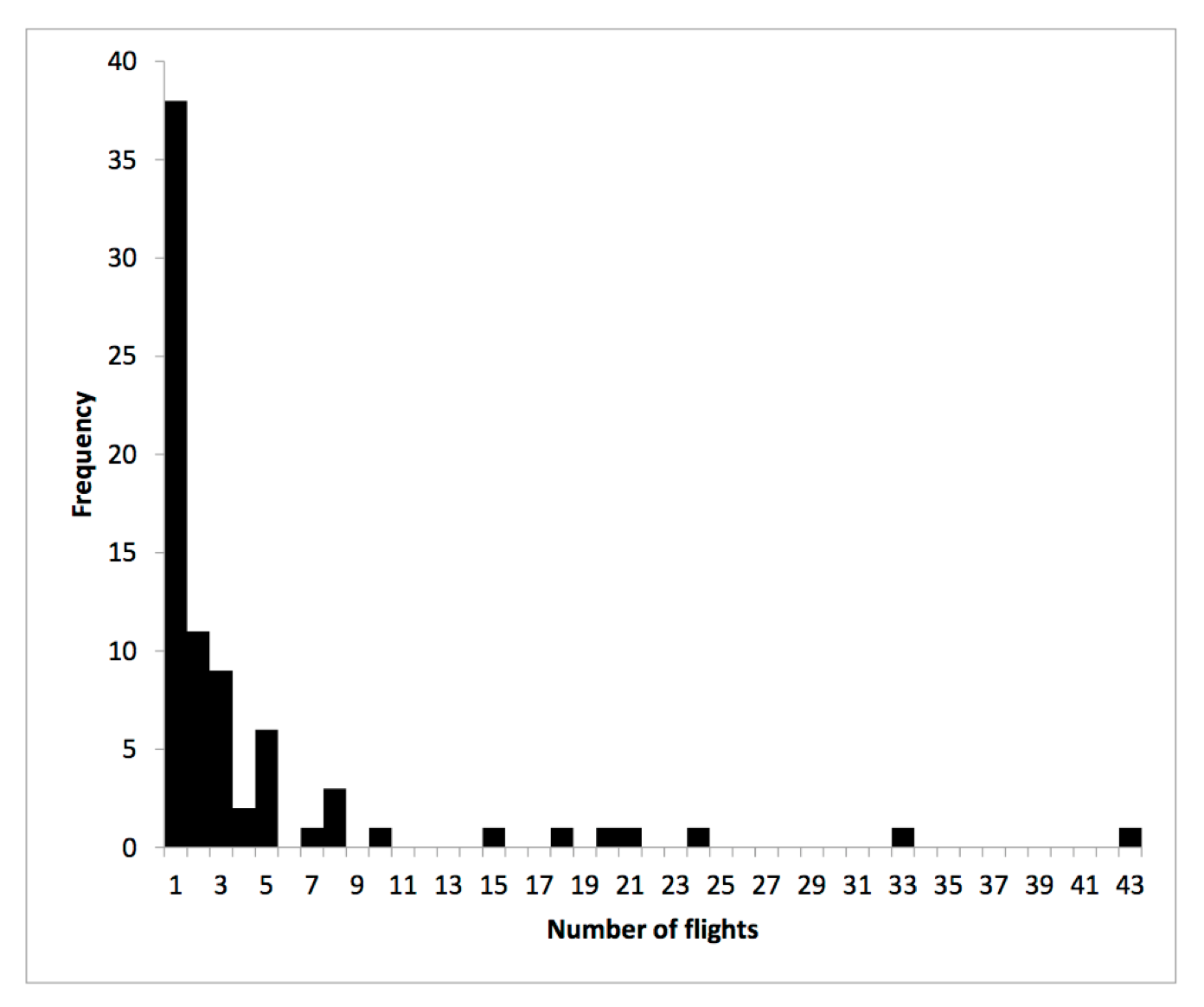
It’s a classic power law/Paretian distribution. From the data, I know that the mean number of flights arriving and departing into a port is 4.4, with a standard deviation (SD) of 7.3.

Let’s then assume that I am working on a particular problem—again, a sample space—where the relevant variables are airports in Australia and the flights that arrive and depart from them. Without knowing anything about any of the individual places, it would be difficult to predict with any confidence which of the towns are likely to serve as the connecting hubs. The mean of 4.4 and SD of 7.3 doesn’t give me much confidence. If other variables were added into the mix, such as the provision of limited information about a possible upcoming terrorist activity in Australian airspace at some unspecified point in the future, and perhaps a possible La-Nina influenced increase in cyclonic activity in Australia’s north during the next monsoon, projections– or probabilities-based realms would not serve me particularly well.

Instead, I would turn to the possibilities-based realm to help me work with—but not necessarily solve—the problem.

‍

Are Gaussian and Paretian Worlds Mutually Exclusive?

To reinforce an earlier point from the above, rather than giving you two different discrete examples—one of the Gaussian World, one of the Paretian World—I deliberately gave you two examples which occur in the same context (i.e. Australia). This is important, because we must always avoid falling into the trap of binary logic: of thinking something is either one thing or the other, but never both at the same time.

Rather, being able to hold paradox and work with multiple contexts at the same time is absolutely critical when working across multiple domain types. Indeed, the realities of our lives are that Gaussian Worlds nest within Paretian ones, and vice-versa.

Finally, and critically, we must also be able to understand that when working in the complex Paretian World, understanding the concept of fractals (which we shall cover in the second-to-next piece)—where the same dispositional dynamics occur at multiple scales across the same system—and how they relate to Paretian distributions and power laws is crucial.

‍

So what?

In case you’re still asking “so what?”, there are a number of things that you could take away from an understanding of Gaussian and Paretian worlds.

For example, if you’re trying to understand how it is that the world’s 26 wealthiest people have a combined net worth which is the same as the combined net worth of world’s poorest 3.5 billion people, the Paretian World is your answer.

Or perhaps you’d like to know why it is that football player Cristiano Ronaldo has a total of160 million Instagram followers and you have a total of 16. Again, the Paretian World is your answer.

Or perhaps you’d like to know why it is that Facebook and Google dominate your digital life, and not Myspace and AltaVista. Again, the Paretian World is your answer.

But specifically in terms of organisations, the overall point I’m making is that the traditional approach to organisational leadership, management and strategy is based on the false belief that only the Gaussian World exists.

Think about the following independent-additive processes that regularly occur in organisations, and in particular think not only about how these processes to occur in isolation from one another (and also from the broader systems to which they belong), but also how they are each treated as stand-alone objects and things:

• strategy development
• leadership development
• culture change
• annual budgeting
• risk management
• restructuring
• team-building

All of these business processes are based upon good and best practice. All of these business processes are based on thinking from 20-30 years ago when the world was less-connected. All of these business processes are ex ante and are devoid of awareness and visibility of the organisational landscapes that give the organisation its evolutionary potential in the here and now.

In short, all of these business processes are based on the false belief that only the Gaussian World exists.

When that belief changes to an understanding that the Paretian World is not only very real but also one in which your organisation inhabits, it becomes apparent how desperately the above processes are in need of a radical overhaul.

At the core of the radical overhaul must be the understanding that these processes cannot be viewed as isolated objects*. The understanding must reinforce that when objects become connected, their nature changes.

* But of course you’ll need to have more than just an understanding. You also need to have the appropriate set of tools (and by appropriate I mean complexity-based tools, noting that there are some very good ones out there) to help you make the radical change and ensure its continued survival and evolution. 90 % of my work these days is in helping build the understanding and then teaching folks how to use the tools in the complex domain. The Cynefin Framework to which I referred earlier is but one of a broader and rapidly emerging suits of tools that I use.

And of course, it’s not just business processes that need to be reconsidered through a lens of connection and multiplacitivability, but also people.

And indeed, if there is to be one key takeaway from your time invested in reading this piece, the following is it:

People have always been connected, but the internet has radically changed the ways and the speeds with which people connect these days.

Considering the traditional way in which people in organisations are treated as isolated and independent objects—and remembering Joshua Cooper Ramos’s suggestion that “connection changes the nature of an object”—you need to begin to think about how connection has changed the nature of people in organisations*.

* In particular, think about the ways in which Human Resources has traditionally understood people as objects, and the business processes put in place which sustain this understanding. Human Resources is traditionally rooted in the Gaussian World, and tends to ignore the realities of the Paretian World.

The staggering finding of network science in the early 2000s that all human social systems are scale free and Paretian in nature and not random and Gaussian has completely changed the game for organisations.

I can’t stress this enough: there are huge ramifications for the majority of organisations currently undergoing transformation and cultural change who have limited awareness that whilst people are (in a physical sense) additive-independent and linear, they are multiplacitive-interdependent and non-linear in the way that they interact with and relate to one another, which in turn makes culture (as an emergent property of a complex social system) multiplacitive-interdependent and non-linear.

‍

Next Time: Networks

It is sometimes said that the Gaussian World privileges stability, structure, objects and permanent states of being whilst the Paretian World privileges instability, dynamism, fields and ever-changing states of becoming. The ramification for organisations of this is that when we view them in the Paretian context, recognising them as objects is mistaken: instead we need to understand them as processes of organising*.

* Which is why Deleuze, Guattari and De Landa’s Assemblage Theory is so relevant.

This brings us to a timely conclusion, and a link to our next theme to explore: networks. Closely linked to scale free Paretian Worlds, networks are the forever-evolving structures which complex systems exhibit, and it’s the next of the 12 themes that we’ll look at.

‍